Nonlinear Curve Fit LM VI
- Updated2025-03-14
- 5 minute(s) read
Uses the Levenberg-Marquardt algorithm to determine the set of parameters that best fit the set of input data points (X, Y) as expressed by a nonlinear function y = f(x,a), where a is the set of parameters. You must manually select the polymorphic instance to use.
Inputs/Outputs
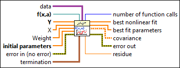
 data
—
data
—
data specifies static data that the user-defined function needs at run time.  f(x,a)
—
f(x,a)
—
f(x,a) is a reference to the VI that implements the fitting model. a is the set of parameters LabVIEW calculates. Use the VI template located at labview\vi.lib\gmath\NumericalOptimization\LM model function and gradient.vit to create the VI from a template.  Y
—
Y
—
Y specifies the array of dependent values, or the observations. The number of input points must be greater than zero.
X
—
X specifies the array of independent values. The number of input points must be greater than zero.
Weight
—
Weight is the array of weights for the observations Y. If Weight is unwired, this VI sets all elements of Weight to 1. If Weight has fewer elements than Y, this VI pads the end of Weight with ones so that the length of Weight equals the length of Y. If Weight has more elements than Y, this VI ignores the extra elements at the end of Weight. If an element in Weight is less than 0, this VI uses the absolute value of the element.
initial parameters
—
initial parameters specifies the initial guess for best fit parameters. The length of initial parameters must equal the length of a in f(x,a). The success of the nonlinear curve fit depends on how close the initial parameters are to the best fit parameters. Therefore, use any available resources to obtain good initial guess parameters to the solution before you use this VI.  error in (no error)
—
error in (no error)
—
error in describes error conditions that occur before this node runs. This input provides standard error in functionality.  termination
—
termination
—
termination specifies the stopping conditions for the fitting process.
 number of function calls
—
number of function calls
—
number of function calls returns the number of times LabVIEW called f(x,a) during the fitting process.  best nonlinear fit
—
best nonlinear fit
—
best nonlinear fit returns the y-values of the fitted model that correspond to the independent values in X.
best fit parameters
—
best fit parameters returns the array of parameters that minimizes the weighted mean square error between the best nonlinear fit and the observations in Y.  covariance
—
covariance
—
covariance returns the matrix of covariances. Cjk is the covariance between a[j] and a[k]. c[jj] is the variance of a[j]. This VI generates the covariance, C, according to the following equation: C = (0.5D)^–1 where D is the Hessian of the function with respect to its parameters.  error out
—
error out
—
error out contains error information. This output provides standard error out functionality.  residue
—
residue
—
residue returns the weighted mean square error between the best nonlinear fit and Y. |
 max iteration
—
max iteration
—
 tolerance
—
tolerance
—
This VI uses the Levenberg-Marquardt method to calculate the best fit parameters that minimize the weighted mean square error between the observations in Y and the best nonlinear fit. The following equation defines the curve model:
y[i] = f(x[i], a0, a1, a2, …)where a0, a1, a2, … are the Parameters.
The Levenberg-Marquardt method does not require y to have a linear relationship with the Parameters.
The Hessian matrix is a common matrix in numerical optimization methods, such as the Newton method. To avoid the weakness of the singular Hessian matrix, the Levenberg-Marquardt method adds a positive definite diagonal matrix to the Hessian matrix. This positive definite diagonal matrix is the main difference between the Levenberg-Marquardt method and the Gauss-Newton method. Refer to Numerical Optimization in the Mathematics Related Documentation topic for more information about the Levenberg-Marquardt method.
You can use the nonlinear Levenberg-Marquardt method to fit linear or nonlinear curves. However, when you fit a linear curve, the General Linear Fit VI is more efficient than this VI. You must verify the results you obtain with the Levenberg-Marquardt method because the method does not always guarantee a correct result.
Examples
Refer to the following example files included with LabVIEW.
- labview\examples\Mathematics\Fitting\Ellipse fit.vi
- labview\examples\Mathematics\Fitting\Sum of 3 Gaussians with offset fit.vi
- labview\examples\Mathematics\Fitting\Gaussian surface with offset fit.vi